Previous puzzle: Puzzle Piece 5: The Doppler Challenge
The only potentially really weird thing in quantum mechanics in my opinion is the concept of “entanglement”. After reading and re-rereading lots of papers on it, at some point I decided that the best way to really understand the problem is to write a computer simulation.
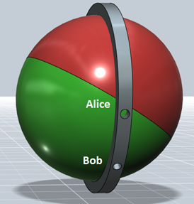
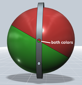
But first, let me try to explain the problem in simple terms – using a similar model as Caroline Thompson’s chaotic ball. Imagine a colored ball, one side red and one side green. A ring with holes is attached. We can rotate the ball in any direction, and when it stops, two players Alice and Bob each peek through a hole and check what color they see. Then they write down two things:
- how far apart he holes were (in degrees, such as 45 degrees),
- whether they agreed on the color or not
(if both saw red or both saw green, then they agreed)
In the first example, they both see green – so they agree. The angle is say 45 degrees between the holes.
Now we repeat this game many times, for different random orientations of the ball. You can see that if the red/green border falls between the holes, they won’t agree, and otherwise they will agree. After say 1000 such experiments, we change the angle between the holes to one of:
- 0 degrees (just one hole – both use the same 🙂
- 45 degrees
- 90 degrees
- 180 degrees
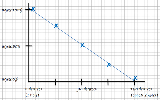
Obviously, for 0 degrees, Alice and Bob always agree on the color, since they both look into the same hole :-):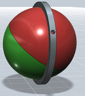
For 180 degrees, they never agree (since the holes are completely opposite).
Finally, we plot the result: for each angle between the holes (such as 0 degrees), we count the percentage of how often we agreed (nr of agreements / total observations). This will result in the typical shape like this – a straight line down:
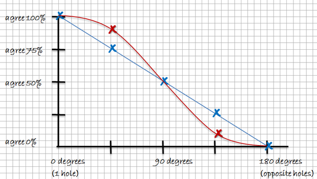
So… what is special about that? So far, absolutely nothing :-). The thing is, if you do this with photons (two photon beams that have the same or opposite polarization, for instance), then you get the red curve – a cosine shape:
Before we jump to conclusions and exclaim that this is proof of entanglement, let’s see if we can reproduce this result with our red/green ball. And yes, we can actually quite easily do it!
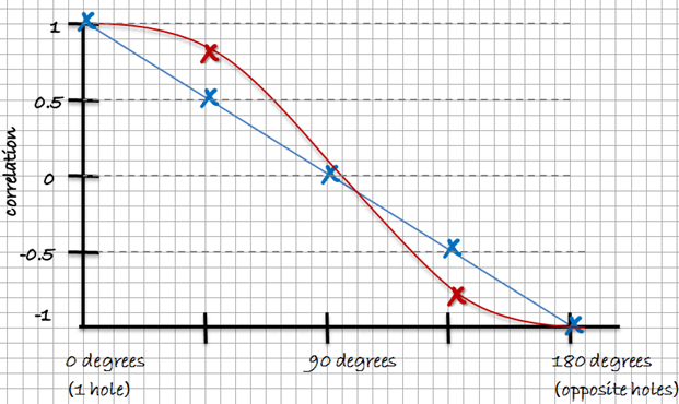
First, just to be a bit more accurate, we don’t express the “agree” in percent, but in correlation. 0% agree means a correlation of –1, 50% agree means 0 correlation, and 100% agree means a correlation of 1:
Now we change the rules of the game just a tiny bit: whenever we look into the hole and see both colors (red and green), like in the image below, then we have the right to say “I don’t know!”
In that case, we don’t record a value (or just a question mark). To make this even more like the quantum mechanics result, we say “I don’t know” more often when we see both colors about the same amount, like in this image:
And we decide to call the color more often if one color clearly dominates (even though both colors are visible):
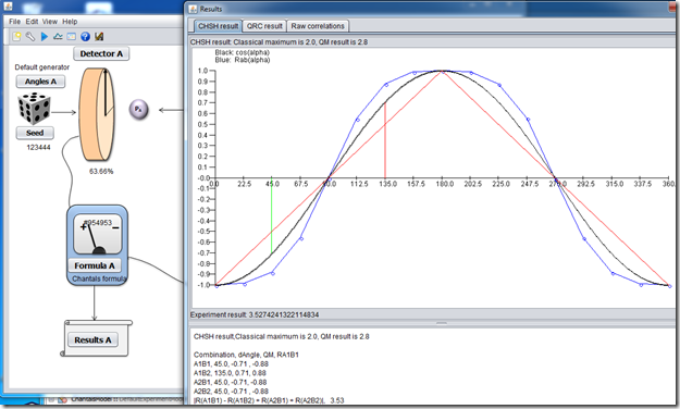
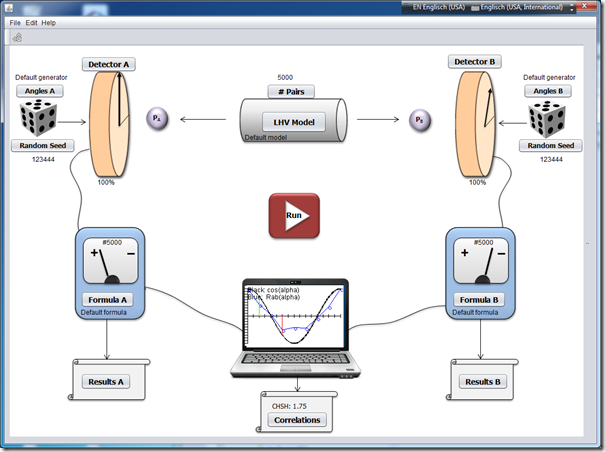
What does this change? Below is the result of a computer simulation that I wrote that you can download from GitHub: https://github.com/chenopodium/tango, which simulates such a game (in this example we can get even a “better” result than in QM). This game is called the “detection loophole” if you read papers on this (but there are other interpretations as well).
Instead of a red/green ball, we have two photon beams (PA and PB), which are created in a way that one beam is polarized up/down, and the other one is polarized left/right. This can be done with a beam splitter – similar to a prism. So we know that if one of the photon beams is up/down polarized, then the other side is left right polarized, and vice versa (of course we can make it so that there is a random angle to the whole thing, like in the example with the ball). These two beams are now called “entangled”. The reason is that the system can be described with one mathematical formula (since the polarization is correlated).

The detector is like our holes, where we decide if we measure the same polarization or not (up or down instead of red or green). Also, our detector can say “I don’t know” in this model.
You can click on the various images and change the rules of the game a bit, and see what the resulting correlation curve looks like. One rule you can change for instance is how large the “holes” are – basically how likely we are to say “I don’t know”. We know from experiments that we do detect at least 70-80% of the pairs (approximately), so we know approximately how often we can say “I don’t know” and still get results that match the actual QM experiments with photons.
For those who prefer the programming language R over Java, there is also an R simulation of the same type of “game”: http://rpubs.com/chenopodium/detection1. (Thanks Richard Gill for the help!)
The additional wavy line on top shows how often we did make the call (and how often we said “I don’t know”). In the chart below, we more had “no detection” around 90 degrees than at 0 degrees – and this is the reason why we get the cosine shape.
Where’s the Magic?
You are probably wondering… so where exactly is the magic, and what is all the fuss about entanglement? Well, if it turns out – and that is actually not known yet! – that we indeed are not measuring all pairs at all angles the same number of times, then there is in fact no magic. Then the only “entanglement” is in the mathematical formula, and in the fact that we know that the beams angle is correlated at the source – and nothing else (or at least, not in those kinds of experiments). Of course we can debate possible reasons why we don’t measure all photons. In fact, it might well just be the way how polarizers work: the intensity of the beam that passes the polarizer is a function of the angle, known as Malus Law. Professor Croft has written a simulation based on exactly that, and shown that the violation can be explained simply based on that.
This is just one tiny part of this huge discussion, for more information, please check out the links below, in particular this blog:
http://challengingbell.blogspot.ch/
If someone can prove that we do indeed measure all photons equally at all angles (and also produce an equal number of photons for each angle!), then yes, there is something weird going on. And then we need to seriously think about what this means (you can pick one of the weird models: faster then speed of light communication, some kind of connection in another dimension, parallel universes etc…)
However, until that day, I am not getting too excited about it :-).
First puzzle: Puzzle Piece 1: Optical Black Holes and Particles of Sound
Links
Papers and Information Links
- http://philoscience.unibe.ch/documents/TexteHS10/bell1964epr.pdf
- http://www.drchinese.com/David/Aspect.pdf
- http://cms.unige.ch/gap/optics/wiki/_media/publications:bib:annphys_9_831.pdf
- http://www.drchinese.com/David/EPR_Bell_Aspect.htm
- http://en.wikipedia.org/wiki/Loopholes_in_Bell_test_experiments
Links to web pages (alternative models, blogs etc):
- Prof. Croft’s simulation based on the Malus Law:
http://www.life.illinois.edu/crofts/papers/Epistemology_and_QM_11-14-08.pdf - Chaotic Ball: http://arxiv.org/abs/quant-ph/9611037
- http://freespace.virgin.net/ch.thompson1/intro.htm
- Challenging Bell Blog: http://challengingbell.blogspot.ch/
http://challengingbell.blogspot.ch/2014/02/new-models-by-richard-gill-and-chantal.html - Joy Christian: http://arxiv.org/abs/1211.0784
- http://freespace.virgin.net/ch.thompson1/
- http://quantummechanics.mchmultimedia.com/
Simulations that I wrote or participated in:
- Java: Tango, an EPR playground to try multiple models): https://github.com/chenopodium/tango
- Java: older NetBeans implementation: https://github.com/chenopodium/EPR
- R: detection loophole: http://rpubs.com/chenopodium/detection1 (with help from Richard Gill)
- R: model for Joy Christian: http://rpubs.com/chenopodium/joychristian
- R: Gisin experiment: http://rpubs.com/chenopodium/gisin1
- R: another version of Joy Christians model: http://rpubs.com/chenopodium/joychristian
- Java, Joy Christians model: http://challengingbell.blogspot.ch/2013/09/a-parallelized-3-sphere-based-simulation.html
https://github.com/chenopodium/JCS - Java, another version of Joy’s model: https://github.com/chenopodium/JCS2
- Java, for Bryan Sanctuary: http://challengingbell.blogspot.ch/2013/05/a-local-realistic-simulation-of-epr.html
- Java (simple, tiny simulation): : https://github.com/chenopodium/Eberhard
The purpose of this simulation is to check if a local realistic model can explain Bell type experiments. If the detection efficiency is greater than in the experiments (such as Guistina 2015), then it means a LHV is still possible. If the experiment has better detection efficiency than the critical efficiency (please see https://arxiv.org/ftp/arxiv/papers/1411/1411.6053.pdf), then a LHV can no longer explain it.
- Java (simple, tiny simulation): https://github.com/chenopodium/Coincidences
Investigation of the coincidence “loophole” in Bell type experiments. The purpose of this simulation is to check if a local realistic model can break the CH inequality (J), as in the Giustina 2015 experiment. This simulation just focuses on the coincidence “loophole”, but not using some “cheap” trick. The goal is to do something similar as is done in the experiment.Based on Jan-Åke, the experiment used fixed time windows, so this simulation is doing the same.
Other simulations:
- in Java Script: http://libertesphilosophica.info/eprsim/EPR_3-sphere_simulation_test5m.html
- Python: https://github.com/minkwe/epr-simple/
- c# simulation: http://sourceforge.net/projects/epr-bohm/
